folije za Libijce

Veljko Milutinovic

DPS: Basics

vm@etf.rs

FIGHTING THE NEGATIVE EFFECTS
OF
CONTROL DEPENDENCIES: A SUMMARY

Problem:
Control dependencies limit the available ILP.

Why?
In classical architectures, branching means resetting the ILP to 0.

Techniques to overcome the negative effects of control dependencies:

ELIMINATION through PREDICATED EXECUTION

Essence:

Conversion of control dependencies into data dependencies.

CONCEALATION through RUN-TIME or COMPILE-TIME TRANSFORMATIONS

Essence:
Execution of control-independent code in parallel,
while waiting for control transfer to take place
(multiple execution streams or delayed branch execution).

PREDICTION through SPECULATION

Essence:
Speculating the outcome of branch instructions,
doing speculative execution, and validation or reexecution.

Important about fighting the negative effects of data dependencies:

Strategies - the same! Tactics - quite different!

FIGHTING THE NEGATIVE EFFECTS

OF

DATA DEPENDENCIES

Problem:
Data dependencies limit the available ILP.

Why?
In classical architectures,
an instruction can not be executed,
until after the results are produced,
by all previous instructions that the current one is data-dependent on.

Techniques to overcome the negative effects of data dependencies:

1. ELIMINATION
through dependence collapsing by fusing [e.g., Montoye90],
or by other techniques [e.g., Milutinovic98].

2. CONCEALATION
through run-time efforts [e.g., Smith95],
or compile-time efforts [e.g., Hwu95].

PREDICTION
through data value prediction [e.g., Lipasti96],
or data address prediction [e.g., Gonzalez97].

SELECTED REFERENCES

[Gonzalez97] Gonzalez, J., Gonzalez, A.,

Speculative Execution via Address Prediction and Data Prefetching,
Proceedings of the 11th ACM 1997 International Conference on Supercomputing,
Vienna, Austria, July 1997, pp. 196-203.

[Hwu95] Hwu, W.W., et al.,

Compiler Technology for Future Microprocessors,
Proceedings of the IEEE, Vol. 83, No. 12, December 1995, pp. 1625-1640.

[Lipasti96] Lipasti, M.H., Shen, J.P.,

Exceeding the Dataflow Limit via Value Prediction,
Proceedings of the 29th International Symposium on Microarchitecture - MICRO-29,
Paris, France, December 1996, pp. 226-237.

[Milutinovic98] Milutinovic, V.,

"Surviving the Design of Microprocessor and Multimicroprocessor Systems:
Lessons Learned," IEEE CS Press, Los Alamitos, California, 1998.

[Montoye90] Montoye, R.K., Hokenek, E., Runyon, S.L.,

Design of the IBM RISC System/6000 Floating-Point Execution Unit,
IBM Journal of Research and Development,
Vol. 34, No. 1, January 1990, pp. 59-70.

[Smith95] Smith, J.E., Sohi, G.S.,

The Microarchitecture of Superscalar Processors,
Proceedings of the IEEE, Vol. 83, No. 12, December 1995, pp. 1609-1624.

MAJOR TECHNIQUES TO OVERCOME

THE NEGATIVE EFFECTS OF DATA DEPENDENCIES

DEPENDENCE COLLAPSING
Combining the data-dependent instructions into a single one,
using a fused functional unit [e.g., Montoye90].

PARALLEL EXECUTION OF NON-CONSEQUTIVE DATA-INDEPENDENT INSTR'S
While waiting for needed data to get ready,
other instructions which are data-independent
can be executed in parallel,
through run-time "shuffling" of instructions [e.g., Smith95],
or compile-time "shuffling" of instructions [e.g., Hwu95].

DATA VALUE PREDICTION
Speculating the result of a data-producing instruction
(based on past behavior of previous instances of the instruction)
and using the speculated (predicted) value in speculative execution,
which is later (after the real result becomes available)
either validated (with NO LOSS of additional cycles),
or reexecuted (with a LOSS of additional cycles).

SOME DATA VALUE PREDICTION TECHNIQUES

Problem:
Predicting 1 out of 2^W outcomes
(not 1 out of 2 outcomes, like in branch prediction)

Some important techniques:

Dynamical instruction reuse [Sodani97]
Last outcome predictor [Lipasti97]

Stride based predictor [Wang97]

Two level predictor [Wang97]

Hybrid predictors [Wang97]

References:

[Sodani97] Sodani, A., Sohi, G.S.,

Dynamic Instruction Reuse,
Proceedings of the 24th Annual Int'l Symposium on Computer Architecture - ISCA-97,
Denver, Colorado, June 1997, pp. 194-205.

[Wang97] Wang, K., Franklin, M.,

Highly Accurate Data Value Prediction Using Hybrid Predictors,
Proceedings of the 30th Annual Symposium on Microarchitecture - MICRO-30,
Research Triangle Park, North Carolina, December 1997, pp. 281-290.

HOW FREQUENT ARE
THE VALUE-PRODUCING INSTRUCTIONS?

Program	%
go	79
compress	74
m88ksim	72
li	69
gcc	57

Table1: Percentage of Value-Producing Instructions (Dynamical Statistics)

The DYNAMICAL INSTRUCTION REUSE Predictor

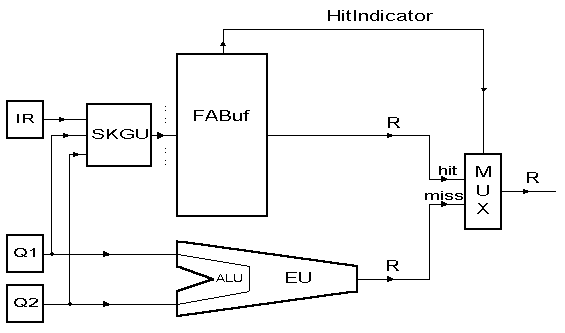
Essence:
No prediction - Only operand value detection and result reuse!
Potentially useful for long latency operations,
because cycles for the execution part of the current instruction are saved.

Figure1: Block Scheme of the Dynamical Instruction Reuse Predictor

Legend:

ALU - Arithmetic and Logic Unit
SKGU - Search Key Generator Unit
EU - Execution Unit
FABuf - Fully Associative Buffer
HitIndicator - Indicator of the Hit in the Fully Associative Buffer
Qi - Operand #1 (i=1,2)
R - Result

Result:

If a 1024-entry FABuf is used,
the execution part can be skipped
in about 33% of data-producing instructions (dynamical statistics).

The LAST OUTCOME Predictor

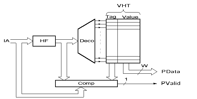
Essence:
Predicting the same value as the one produced
when the same static value-producing instruction was executed last time.
Remember that only a subset of instructions are data-producing!

Figure2: Block Scheme of the Last Outcome Predictor

Legend:

Comp - Comparator
Deco - Decoder
HF - Hash Function
IA - Instruction Address
PData - Predicted Data (W bits)
PValid - Prediction Valid indicator (one bit); just the VHT hit
Tag - Tag storing the identity of the currently mapped instruction
VHT - Value History Table
Value - Value produced during the last execution

of the currently mapped instruction

Result:

For the PowerPC architecture and the SPEC applications,
prediction accuracy is equal to:

49% - for the last ONE value, and
61% - for the last 4 values stored (predictor able to pick the right value)

CRUCIAL DESIGN PARAMETER: DATA VALUE LOCALITY

Problem:
How much history to use for speculation/prediction?

Trade-offs:

Too little history - poor prediction accuracy
Too much history - high hardware and time overheads

Register value locality for a history depth of 16:

Architecture - MIPS R2000
Applications - SPEC'92

Program	%
go	73
compress95	56
m88ksim	91
li	81
gcc	75

Table2: Percentage of Eligible Instructions Reusing 1 of the Last 16 Values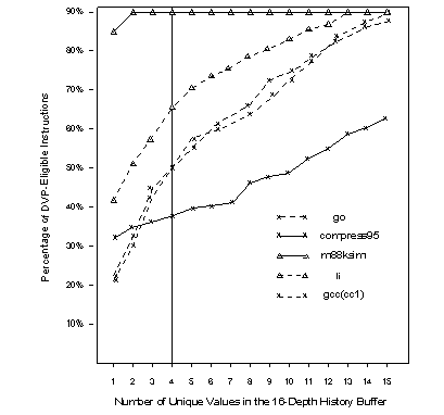

How many of the 16 values are unique?

Figure3: Number of Unique Values in the Last-16-Buf of Eligible Instructions (Cumulative Distribution)

X - Number of unique values in the last-16-buf of eligible instructions
Y - Percentage of register result producing instructions
with X or less unique values

Conclusions[Wang97]:

Case X=1 taken care of by the LAST OUTCOME predictor.
From 22% to 85% of instructions have all their last 16 results the same.

Case X=4 needs a more accurate predictor (knee is at approximately 4).
From 38% to 91% of instructions have 4 or fewer unique values in the last-16.

The STRIDE BASED Predictor

If results vary by a constant stride
then it is easy to predict the result of the next instance of the instruction.

Works well because a relatively large percentage of instructions include:
a. Loop controling variables
b. Array stepping variables

So far used successfully for data prefetching!

Figure4: Block Scheme of the Stride Value Predictor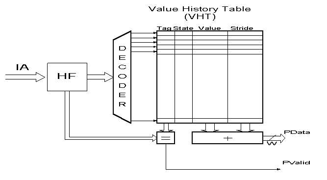

Fields:
TAG = {subset/transform(AddressBits)}
STATE = {Init, Transient, Steady}
VALUE = {LastValueEncountered}
STRIDE = {Dj - Dk}; j=k+1, k=1,2,...

The Stride Detection Phase

At the first execution instance of an instruction - NO prediction is made;
when the instruction produces its result - an entry is allocated in the VHT:

The result D1 is stored into the VALUE field of the allocated entry
The STATE field of the entry is set to {Init}

On the next instance of the same instruction,
if STATE={Init} then again NO prediction is made;
however, it is assumed that the stride value is calculatable
after the second instance of an instruction,
and the following computation is done:

S1=D2-Value(VHT)

S1 - Stride
D2 - Value generated by the second instance of the instruction
Value(VHT) - Value generated by the first instance (D1)

After the computation is completed, the following updates are done:

VALUE={D2}
STRIDE={S1}
STATE={Transient}

If STATE={Transient} then still NO prediction is made
on the next instance of the same instruction;
however, it is assumed that the time has come to declare that

A STABLE STRIDE DOES EXIST
IF THE NEXT RESULT CREATES THE STRIDE
WHICH IS THE SAME AS THE ONE IN THE VHT.

The following calculation is done:

S2=D3-Value(VHT)

The following updates are done:

VALUE ={D3}
STRIDE={S2}
STATE =

{Steady} if S2=S1
{Transient} if S2<>S1 - no change of the STATE field

While STATE={Steady} predictions are done by adding [VALUE]+[STRIDE].

When Sj <> Sk, j=k+1, then STATE={Transient} and prediction STOPs.

After STATE={Steady}, then prediction RESUMEs.

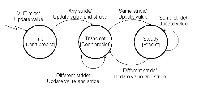
Figure5: State Transition Diagram of the Stride Value Predictor

The TWO LEVEL VALUE Predictor

Enabling assumption:
A substantial percentage of dynamic instructions
have 4 or less unique values
in their most recent history.

Minimal complexity:
Obtained by storing 4 most recent unique values
for EACH instruction
and by doing a binary encoding of these 4 outcomes.

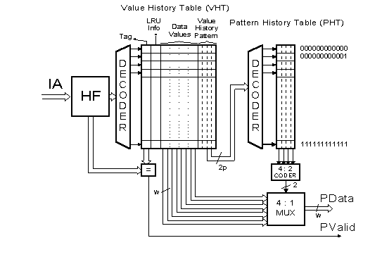
Figure6: Block Scheme of a Two Level Value Predictor

The VHT (of the first level) has four fields:

TAG - Business as usual
DATA - Four subfields for up to four recent unique values;

the four values are associted with the encoding {00,01,10,11}

LRU - Keeping track of the order in which the 4 data values were seen;

when the fifth value appears, the least recently seen value goes out

VHP - Value History Pattern;

the last P outcomes are kept for each instruction in VHT

in the form of a pattern which is 2P bits long

The PHT (of the second level) has one field:

There are 2^2P entries in the PHT.
For each PHT entry, the next outcome likelihood is recorded,
via four independent up/down counter values:
{C1, C2, C3, C4}

When a prediction is to be made for an instruction:

The appropriate VHT entry is selected.
The TAG field is checked to see if the entry corresponds to current instr.
If yes, the VHP value is used to select the PHT entry.
The maximum of the 4 counter values is selected,
and the corresponding value is declared as PREDICTED VALUE.
If there is a tie,
either the last outcome related value is selected,
or one of the values is selected on random.

Note that prediction is made only if the maximum is above a threshold.
If it is below the threshold, no prediction is made.

Updating of the VHT entry:

a. Contents get shifted left by 2 bits.
b. New outcome is entered into the bits left vacant.

Updating of the PHT entry:

a. Selected counter (corresponding to the correct outcome)
gets incremented
by 3 (or less, if 3 generates the saturation).
b. All other counters get decremented by one (unless they are zero).

The HYBRID Predictor

No single scheme provides good prediction for every benchmark!
Solution: A hybrid predictor
Solution of [Wang97]:

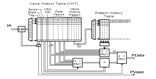Combination of TWO-LEVEL and STRIDE-BASED predictors.
The VHT includes two additional fields: STATE and STRIDE

Figure7: Block Scheme of a Hybrid (Two-Level and Stride-Based) Predictor

Prediction Algorithm:

a. The appropriate VHT entry is selected and the TAG field is checked.
b. In parallel,
the VHP (of Two-Level) and the STATE (of Stride-Based) fields are read out
c. If the selected PHT entry has the maximum count value above the threshold,
then the two-level predictor makes prediction;
otherwise,
the stride-based predictor makes prediction,
unless the STATE<>{Steady}, in which case no prediction is made.

Performance Evaluation:

Conditions assumed:

(i) MIPS-I ISA (integer instructions only)
(ii) SPEC'95 (integer suite only)

Default parameters:
(i) 100 million instructions or till completion (whichever comes first)
(ii) VHT with 4K direct-mapped entries
(iii) PHT with 4K entries (counters saturate at 12; threshold equal to 6)

Metrics used, relatively to the total # of DVP-eligible instructions:
(i) Percentage of instructions correctly predicted
(ii) Percentage of instructions misspredicted
(iii) Percentage of instructions not predicted

Experimental Results:
(i) With the hybrid predictor, one can go up to above 98% (m88ksim)

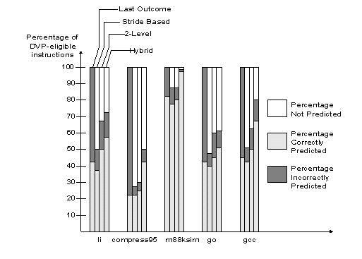
Figure8: Simulation Results for Different Predictors

The TRACE BASED Predictor - Value Oriented

Rationale:
If there are two updates to a register in a trace,
only the second update is live at the end of the trace,
and only it has to be predicted!

Motivation:
Less prediction means
less bandwidth (predictor supplies less data)
and less memory (predictor stores less data)!

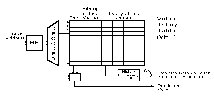
Figure9: Block Scheme of a Trace Based Predictor - Value Oriented

Major differences from instruction based predictors:

(i) The history fields keep track of multiple register values.

(ii) A bit map field is used to store the mapping
from the live register values
to the instructions that produce the values.

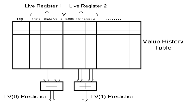
The TRACE BASED Predictor - Stride Oriented

Figure10: Block Scheme of a Trace Based Predictor - Stride Oriented

The TWO LEVEL TRACE BASED Predictor

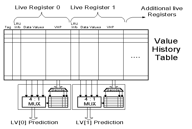
Figure11: Block Scheme of a Two Level Trace Based Predictor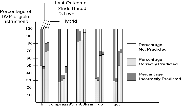

The TRACE BASED Predictor SIMULATION RESULTS

Figure12: Simulation Results for Trace Based Predictors

Veljko Milutinovic

DPS: State-of-the-Art

vm@etf.rs

Veljko Milutinovic

DPS: IFACT

vm@etf.rs